Invert AIA and XRT images for a DEM

This tutorial finds the differential emission measure (DEM) of a coronal jet, how much plasma there is at each temperature along the line of sight through each pixel, from six channels of AIA [Lemen et al., 2012] and the Al_poly filter of XRT [Golub et al., 2007]. AIA alone finds the plasma below about 3 MK well, but it sees so little of the hotter plasma that a DEM from AIA alone can put several times too much there [Athiray and Winebarger, 2024]. XRT is most sensitive to that hot plasma, so the two together constrain the whole range.

The jet is event E of Parker et al. [2022], which the EUV Snapshot Imaging Spectrograph (ESIS) observed on 2019 September 30. Its base is bright enough to saturate a few pixels of XRT in two of the images, so the tutorial uses the image just before them.

The tutorial uses the temperature response of XRT, hinode.xrt.temperature_response(), the uncertainty of each XRT pixel, hinode.xrt.Filtergram.uncertainty(), the response and the uncertainty of AIA from sdo [Boerner et al., 2012], and the regularized inversion of Plowman and Caspi [2020], utu.dem.plowman().

Load the XRT image

The Al_poly image during the ESIS flight just before the first one with saturated pixels, with the visible light which leaks into XRT subtracted. The uncertainty map is loaded too, for the uncertainty of each pixel below.

import numpy as np
import matplotlib.pyplot as plt
import matplotlib.colors
import astropy.units as u
import astropy.visualization
import sunpy.visualization.colormaps
import named_arrays as na
import sdo
import utu
import hinode

images = hinode.xrt.open(
    time_start="2019-09-30T18:06:11",
    time_stop="2019-09-30T18:11:01",
    filter="Al_poly",
    leak=True,
    uncertainty=True,
)

num_saturated = images.saturated.sum(
    axis=(images.axis_detector_x, images.axis_detector_y),
)
first = np.argmax(num_saturated > 0, axis=images.axis_time)[images.axis_time]
xrt = images[{images.axis_time: first - 1}]

xrt = xrt.remove_leak()

xrt.inputs.time.ndarray

<Time object: scale='utc' format='isot' value=2019-09-30T18:08:00.577>

Co-align XRT with AIA

The pointing in the headers of the Level 1 files can be off by about an arcsecond. Yoshimura and McKenzie [2015] cross-correlated the XRT images with AIA, and SolarSoft keeps the result for each image in a database, as the position of the center of the image. hinode.xrt.open() moves the center there by default, as xrt_read_coaldb does in SolarSoft with /aia_cc, which aligns XRT with AIA, and coalignment records how each image was aligned, 1 for the cross-correlation with AIA.

xrt.coalignment

ScalarArray(ndarray=np.int64(1), shape={})

Select a 128-pixel box around the jet.

box = dict(
    detector_x=slice(172, 300),
    detector_y=slice(80, 208),
)

xrt = xrt[box]

Load the AIA images

The image in each channel closest to the middle of the XRT exposure, registered, so that they share one grid of 0.6 arcsecond pixels. AIA takes an image in each channel every 12 seconds, so there is one in the 12 seconds around the middle. JSOC finds the images by the 12-second slot each one belongs to, rather than by when it was taken, so the search also finds images up to 12 seconds outside the range, and only the closest one in each channel is kept.

channels = na.ScalarArray(
    ndarray=[94, 131, 171, 193, 211, 335] * u.AA,
    axes="channel",
)

middle = xrt.inputs.time.ndarray + xrt.timedelta.ndarray / 2

aia = sdo.aia.open(
    time_start=middle - 6 * u.s,
    time_stop=middle + 6 * u.s,
    wavelength=channels,
    register=True,
)

# the time from the middle of the XRT exposure to the middle of each
# AIA exposure
offset = na.ScalarArray(
    ndarray=(aia.inputs.time.ndarray - middle).to(u.s),
    axes=aia.inputs.time.axes,
) + aia.timedelta / 2

aia = aia[np.argmin(np.abs(offset), axis="time")]

# only the part of the disk around the box
aia = aia[dict(
    detector_x=slice(2000, 2270),
    detector_y=slice(1805, 2075),
)]

aia.inputs.time.ndarray

<Time object: scale='utc' format='isot' value=['2019-09-30T18:08:11.120' '2019-09-30T18:08:06.630'
 '2019-09-30T18:08:09.350' '2019-09-30T18:08:04.840'
 '2019-09-30T18:08:09.630' '2019-09-30T18:08:12.630']>

Match the resolution and the pixels

The core of the point-spread function of XRT is about 2 arcseconds wide at half its maximum, and that of AIA about 1.3 arcseconds. Blurring AIA by a Gaussian of the difference in quadrature gives both the same resolution, so that sharp edges, like those of the jet, are as sharp in every channel.

fwhm_xrt = 2 * u.arcsec
fwhm_aia = 1.3 * u.arcsec

sigma = np.sqrt(fwhm_xrt**2 - fwhm_aia**2) / (2 * np.sqrt(2 * np.log(2)))

plate_scale = 0.6 * u.arcsec
x = na.arange(-4, 5, axis="detector_x") * plate_scale
y = na.arange(-4, 5, axis="detector_y") * plate_scale
kernel = np.exp(-(np.square(x) + np.square(y)) / (2 * np.square(sigma)))
kernel = kernel / kernel.sum()

counts = na.convolve(aia.outputs, kernel)

The AIA images are then summed onto the XRT pixels by conservative regridding, which keeps the total signal.

# the corners of the pixels, which registration makes the same in
# every channel
position_aia = aia.inputs.position[dict(channel=0)].to(u.arcsec)
position_xrt = xrt.inputs.position.to(u.arcsec)

weights = na.regridding.weights(
    coordinates_input=position_aia,
    coordinates_output=position_xrt,
    axis_input=("detector_x", "detector_y"),
    axis_output=("detector_x", "detector_y"),
    method="conservative",
)

counts = na.regridding.regrid_from_weights(*weights, values_input=counts)

The variance of each AIA pixel, from sdo.aia.uncertainty(), is summed onto the XRT pixels the same way. That alone would overestimate the noise, since the blur averages neighboring pixels together, and the pixels which straddle two XRT pixels are split between them. How much both average the noise down is found by blurring and regridding white noise of unit variance, and the summed variance is scaled by it. Overestimating the AIA noise would let the inversion fit the six AIA channels better than their noise warrants, and XRT worse.

variance = np.square(sdo.aia.uncertainty(
    counts=aia.outputs,
    wavelength=aia.inputs.wavelength,
))
variance = na.regridding.regrid_from_weights(*weights, values_input=variance)

shape = aia.outputs[dict(channel=0)].shape
noise = na.random.normal(0, 1, shape_random=shape, seed=0)
noise = na.convolve(noise, kernel)
noise = na.regridding.regrid_from_weights(*weights, values_input=noise)
ones = na.regridding.regrid_from_weights(
    *weights,
    values_input=na.ScalarArray.ones(shape),
)

reduction = np.square(noise).mean() / ones.mean()

variance = reduction * variance

reduction

ScalarArray(
    ndarray=0.15628347 ,
    shape={},
)

The regridded AIA images are now in counts per XRT pixel, like XRT, but the responses of AIA below are per AIA pixel. So that the images and the responses can be compared, the images of every channel are divided by the solid angle of an XRT pixel, and each response by the solid angle of its own pixels, which puts both per steradian.

solid_angle_xrt = (xrt.inputs.cdelt.position.x * xrt.inputs.cdelt.position.y).to(u.sr)

intensity_aia = counts / aia.timedelta / solid_angle_xrt
uncertainty_aia = np.sqrt(variance) / aia.timedelta / solid_angle_xrt

intensity_xrt = xrt.outputs / solid_angle_xrt

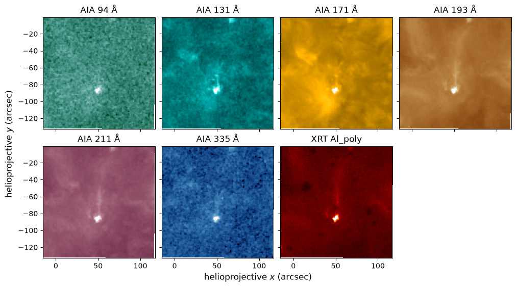
The six AIA channels and XRT on the same pixels.

panels = [
    (f"AIA {c:.0f} Å", intensity_aia[dict(channel=i)], f"sdoaia{c:.0f}")
    for i, c in enumerate(channels.ndarray.value)
]
panels.append(("XRT Al_poly", intensity_xrt, "hinodexrt"))

with astropy.visualization.quantity_support():
    fig, axs = plt.subplots(
        nrows=2,
        ncols=4,
        figsize=(10, 5.5),
        sharex=True,
        sharey=True,
        constrained_layout=True,
    )
    for ax, (title, rate, cmap) in zip(axs.flat, panels):
        na.plt.pcolormesh(
            position_xrt,
            C=rate.value,
            ax=ax,
            cmap=cmap,
            norm=matplotlib.colors.PowerNorm(
                gamma=0.5,
                vmin=0,
                vmax=rate.value.percentile(99.9).ndarray,
            ),
        )
        ax.set_title(title)
        ax.set_aspect("equal")
        ax.set_xlabel("")
        ax.set_ylabel("")
    axs.flat[7].set_axis_off()
    fig.supxlabel("helioprojective $x$ (arcsec)")
    fig.supylabel("helioprojective $y$ (arcsec)")

Uncertainty of XRT

The photon noise of XRT depends on the spectrum, since the photons of each wavelength give a different signal, so uncertainty() needs the ratio of the variance response of hinode.xrt.temperature_response() to its response, \(F\), in DN per photon. It is taken at \(\log_{10} T = 6.3\), near the temperature of most of the plasma in the box.

# log T from 5.0 to 7.5, the temperatures of the inversion
response_xrt = hinode.xrt.temperature_response(
    filter="Al_poly",
    time=xrt.inputs.time.ndarray,
    axis_filter="channel",
)[dict(temperature=slice(0, 51))]

variance_xrt = hinode.xrt.temperature_response(
    filter="Al_poly",
    time=xrt.inputs.time.ndarray,
    variance=True,
    axis_filter="channel",
)[dict(temperature=slice(0, 51))]

logt = np.log10(response_xrt.inputs / u.K)

# F at log T = 6.3
noise_photon = (variance_xrt.outputs / response_xrt.outputs)[dict(temperature=26)]

noise_photon

ScalarArray(
    ndarray=[2.9832121] DN / ph,
    shape={'channel': 1},
)

That is the noise of a CCD which collects all the charge of each photon in the pixel it was absorbed in, before any compression. The noise of these images can be measured instead, from the difference between each image and the next, with ratio_noise(). Away from the jet the Sun barely changes in 18 seconds, so the difference is the noise of the two images, and dividing it by their uncertainties gives a quantity whose variance is the ratio of the measured noise to the predicted noise. The box around the jet and anything bright enough to change are left out, and so are cosmic rays, by clipping at five times the noise.

frames = images.remove_leak()

in_box = na.ScalarArray.zeros(images.outputs[dict(time=0)].shape) > 0
in_box[box] = True

ratio_noise = frames.ratio_noise(noise_photon, where=~in_box)

ratio_noise

ScalarArray(
    ndarray=[0.15269617],
    shape={'channel': 1},
)

The measured variance is only about a sixth of the prediction. The noise of neighboring pixels is also correlated, more strongly inside the 8 by 8 blocks of the JPEG compression of these images than across the edges of the blocks, which shows in the differences of the same pairs of pixels.

# each image and the one after it, if it began soon after with the same
# exposure, as ratio_noise compares them
before = dict(time=slice(None, ~0))
after = dict(time=slice(1, None))
time_frames = frames.inputs.time.ndarray
gap = na.ScalarArray((time_frames[1:] - time_frames[:-1]).to(u.s), axes="time")
change = np.abs(frames.timedelta[after] - frames.timedelta[before])
consecutive = (gap < 25 * u.s) & (change < 0.01 * u.s)

intensity_frames = frames.outputs
variance_frames = np.square(frames.uncertainty(noise_photon))
z = intensity_frames[after] - intensity_frames[before]
z = z / np.sqrt(variance_frames[after] + variance_frames[before])
z = z.to(u.dimensionless_unscaled).value

mean = (intensity_frames[after] + intensity_frames[before]) / 2
clipped = (
    consecutive
    & ~in_box
    & (mean < 10 * u.DN / u.s)
    & (np.abs(z) < 5 * np.sqrt(ratio_noise))
)

left = dict(detector_x=slice(None, ~0))
right = dict(detector_x=slice(1, None))

product = z[left] * z[right]
both = clipped[left] & clipped[right]

index_x = na.arange(0, images.outputs.shape["detector_x"] - 1, axis="detector_x")
edge = index_x % 8 == 7

correlation = {
    "inside a block": product.mean(where=both & ~edge) / ratio_noise,
    "across an edge": product.mean(where=both & edge) / ratio_noise,
}

correlation

{'inside a block': ScalarArray(
     ndarray=[0.4253956],
     shape={'channel': 1},
 ),
 'across an edge': ScalarArray(
     ndarray=[0.28244216],
     shape={'channel': 1},
 )}

We think two effects explain the low noise, and neither is in the uncertainty of Kobelski et al. [2014]. First, the charge each X-ray photon frees in the CCD diffuses across the boundaries of the pixels before it is collected, which lowers the noise of each pixel and correlates it with its neighbors, which is the correlation across the edges of the blocks. Second, the JPEG compression rounds the components of each block which vary fastest across it, which in images this faint removes much of the noise, and correlates the pixels within a block further. Until there is a model of both, the uncertainty of XRT is scaled to the measured noise. It was measured in the quiet Sun, and compression removes less of the noise of a brighter pixel, so it may underestimate the noise in the brightest parts of the jet.

uncertainty_xrt = np.sqrt(ratio_noise) * xrt.uncertainty(noise_photon) / solid_angle_xrt

Temperature response

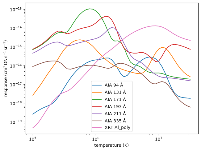
The response of each AIA channel normalized to SDO/EVE, as in the DEM tutorial of sdo, and that of Al_poly at the time of the image, both per steradian like the intensities. The response of AIA is per AIA pixel, whose solid angle is that of the registered pixels. The response of 94 Å includes the empirical correction of Boerner et al. [2014] for the lines near 1 MK which CHIANTI is missing, chiantifix=True; without it the DEM predicts only about half of the 94 Å observed.

The inversion runs from \(\log_{10} T = 5.0\) to 7.5. The far wing of the passband of 335 Å takes in the bright lines of the transition region between 550 and 800 Å, O V 629.7 Å the brightest of them, so 335 Å responds more to plasma at \(\log_{10} T = 5.2\) to 5.4 than at its peak of Fe XVI near 6.4, while the other channels respond to it at less than a fifth of their peaks. A DEM which starts at 5.5 has none of that plasma, and cannot make the 335 Å observed. Below 5.5 the DEM rests mostly on 335 Å, and its shape there on the smoothness of the inversion.

response_aia = sdo.aia.temperature_response(
    wavelength=channels,
    time=aia.inputs.time.ndarray.min(),
    eve=True,
    chiantifix=True,
)[dict(temperature=slice(20, 71))]

solid_angle_aia = (plate_scale**2).to(u.sr)

unit = u.DN * u.cm**5 / u.s / u.sr

outputs_aia = (response_aia.outputs / (solid_angle_aia / u.pix)).to(unit)
outputs_xrt = (response_xrt.outputs / (solid_angle_xrt / u.pix)).to(unit)

response = na.FunctionArray(
    inputs=response_aia.inputs,
    outputs=np.concatenate([outputs_aia, outputs_xrt], axis="channel"),
)

labels = [f"AIA {c:.0f} Å" for c in channels.ndarray.value] + ["XRT Al_poly"]

with astropy.visualization.quantity_support():
    fig, ax = plt.subplots(constrained_layout=True)
    na.plt.plot(
        response.inputs,
        response.outputs,
        ax=ax,
        axis="temperature",
        label=na.ScalarArray(np.array(labels), axes="channel"),
    )
    ax.set_xscale("log")
    ax.set_yscale("log")
    ax.set_xlabel(f"temperature ({response.inputs.unit:latex_inline})")
    ax.set_ylabel(f"response ({response.outputs.unit:latex_inline})")
    ax.legend()

Invert

The intensities and uncertainties of all seven channels, along one axis.

def stack(aia, xrt):
    xrt = na.broadcast_to(xrt, aia[dict(channel=slice(1))].shape)
    return np.concatenate([aia, xrt], axis="channel")

intensity = stack(intensity_aia, intensity_xrt.add_axes("channel"))

Invert every pixel of the box.

dem, chi2 = utu.dem.plowman(
    intensity=intensity,
    uncertainty=stack(uncertainty_aia, uncertainty_xrt),
    response=response,
    axis_channel="channel",
    axis_temperature="temperature",
)

# the median reduced chi squared, which the inversion aims at one
chi2.median()

ScalarArray(ndarray=np.float64(0.9680692603197105), shape={})

For comparison, invert AIA alone too, and find the ratio of the XRT intensity each DEM predicts to the one observed. The emission measure in each step of temperature is the DEM times the step in \(\log_{10} T\).

dem_aia, chi2_aia = utu.dem.plowman(
    intensity=intensity_aia,
    uncertainty=uncertainty_aia,
    response=response[dict(channel=slice(6))],
    axis_channel="channel",
    axis_temperature="temperature",
)

step = 0.05

# the ratio of the XRT intensity a DEM predicts to the one observed
def ratio_xrt(dem):
    predicted = (dem.outputs * outputs_xrt * step).sum("temperature")
    ratio = (predicted / intensity_xrt).to(u.dimensionless_unscaled)
    return ratio[dict(channel=0)]

ratio = ratio_xrt(dem)
ratio_aia = ratio_xrt(dem_aia)

# the median over the box
{
    "AIA + XRT": ratio.median(),
    "AIA only": ratio_aia.median(),
}

{'AIA + XRT': ScalarArray(
     ndarray=1.22856271 ,
     shape={},
 ),
 'AIA only': ScalarArray(
     ndarray=9.01392403 ,
     shape={},
 )}

In most of the box, the DEM from AIA alone predicts 3 to 18 times the XRT intensity observed. AIA sees so little of the plasma above about 4 MK that the smoothest DEM which fits its six channels can have a tail of hot plasma there, which XRT rules out.

Results

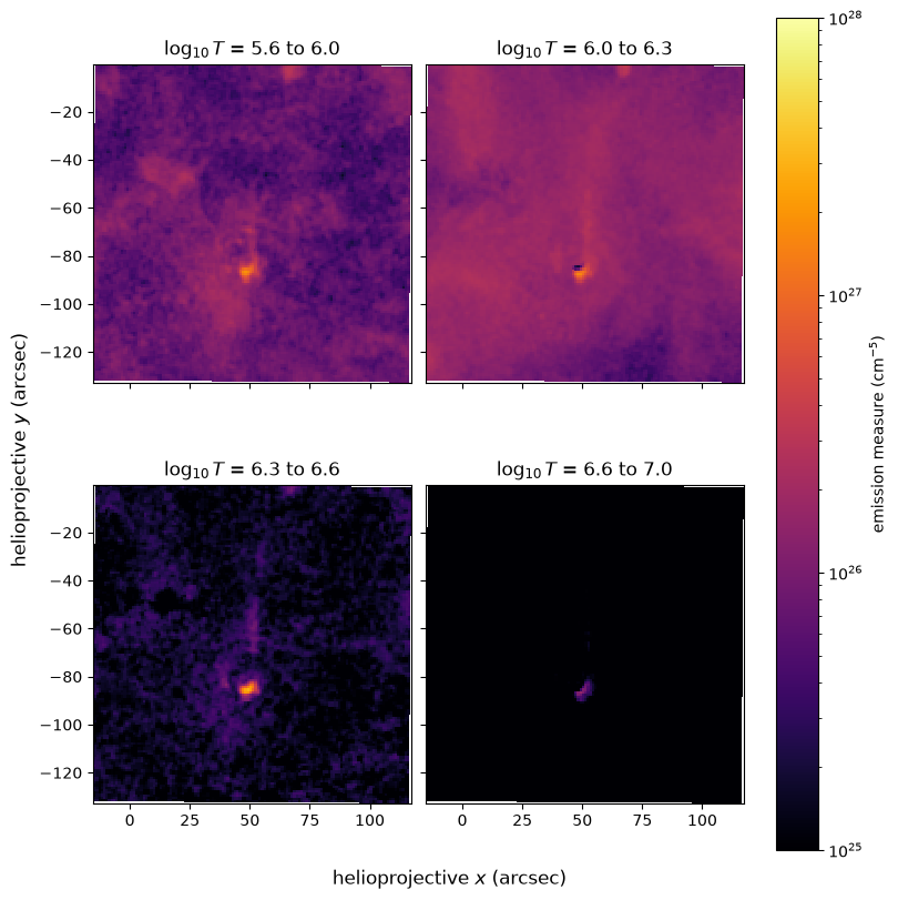
The emission measure in four ranges of temperature, the integral of the DEM over each.

ranges = [(5.6, 6.0), (6.0, 6.3), (6.3, 6.6), (6.6, 7.0)]

em = {
    r: (dem.outputs * step).sum("temperature", where=(logt >= r[0]) & (logt < r[1]))
    for r in ranges
}

with astropy.visualization.quantity_support():
    fig, axs = plt.subplots(
        nrows=2,
        ncols=2,
        figsize=(8, 8),
        sharex=True,
        sharey=True,
        constrained_layout=True,
    )
    for ax, r in zip(axs.flat, ranges):
        mesh = na.plt.pcolormesh(
            position_xrt,
            C=em[r].value,
            ax=ax,
            cmap="inferno",
            norm=matplotlib.colors.LogNorm(vmin=1e25, vmax=1e28),
        )
        ax.set_title(rf"$\log_{{10}} T$ = {r[0]} to {r[1]}")
        ax.set_aspect("equal")
        ax.set_xlabel("")
        ax.set_ylabel("")
    fig.supxlabel("helioprojective $x$ (arcsec)")
    fig.supylabel("helioprojective $y$ (arcsec)")
    fig.colorbar(
        mesh.ndarray.item(),
        ax=axs,
        label=f"emission measure ({em[r].unit:latex_inline})",
    )

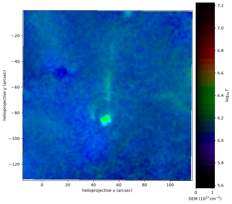
The whole DEM in one false-color image, made with named_arrays.colorsynth, as in the DEM tutorial of sdo. Temperature is mapped onto the visible spectrum, from violet for the coolest plasma to red for the hottest, and each pixel is colored as if the DEM were the spectrum of the light it emits. Every temperature shares one linear scale, up to the 99.5th percentile of the whole DEM, so the brightness of a pixel is how much plasma it has and the color is at what temperature. The plasma around the jet is mostly near 1 MK, which comes out blue, and the base of the jet, at 2 to 3 MK, comes out green. There is almost no red, since XRT allows almost none of the plasma above 4 MK that AIA alone would put there.

constrained = dem[dict(temperature=slice(12, 45))]

# in units of 10^27 cm^-5, so that the colorbar needs no offset
dem_27 = (constrained.outputs / (1e27 / u.cm**5)).to(u.dimensionless_unscaled)

with astropy.visualization.quantity_support():
    fig, axs = plt.subplots(
        ncols=2,
        figsize=(8, 7),
        gridspec_kw=dict(width_ratios=[0.9, 0.1]),
        constrained_layout=True,
    )
    colorbar = na.plt.rgbmesh(
        np.log10(constrained.inputs / u.K),
        position_xrt,
        C=dem_27,
        axis_wavelength="temperature",
        ax=axs[0],
        vmin=0,
        vmax=np.nanpercentile(dem_27, q=99.5),
    )
    na.plt.pcolormesh(
        C=colorbar,
        axis_rgb="temperature",
        ax=axs[1],
    )
    axs[0].set_aspect("equal")
    axs[0].set_xlabel("helioprojective $x$ (arcsec)")
    axs[0].set_ylabel("helioprojective $y$ (arcsec)")
    axs[1].set_xlabel(r"DEM ($10^{27}\,\mathrm{cm^{-5}}$)")
    axs[1].set_ylabel(r"$\log_{10} T$")
    axs[1].yaxis.tick_right()
    axs[1].yaxis.set_label_position("right")

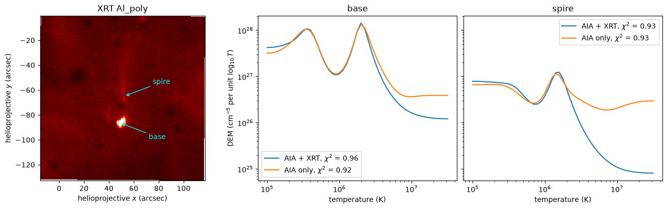
The DEM of the brightest pixel of the base and of a pixel in the spire, from AIA and XRT together and from AIA alone, with both pixels marked on the XRT image. The two agree on the plasma at 1 to 2 MK, and above about 3 MK AIA alone has the tail of hot plasma. At the base both have a second peak, near 0.35 MK, of the transition-region plasma which 335 Å sees.

base = np.argmax(xrt.outputs, axis=("detector_x", "detector_y"))
spire = dict(detector_x=65, detector_y=65)

pixels = dict(base=base, spire=spire)

# the center of each pixel, from its corners
center = position_xrt.cell_centers(axis=("detector_x", "detector_y"))

inversions = [
    ("AIA + XRT", dem, chi2),
    ("AIA only", dem_aia, chi2_aia),
]

with astropy.visualization.quantity_support():
    fig, axs = plt.subplots(
        ncols=3,
        figsize=(13, 4),
        constrained_layout=True,
    )
    na.plt.pcolormesh(
        position_xrt,
        C=intensity_xrt.value,
        ax=axs[0],
        cmap="hinodexrt",
        norm=matplotlib.colors.PowerNorm(
            gamma=0.5,
            vmin=0,
            vmax=intensity_xrt.value.percentile(99.9).ndarray,
        ),
    )
    # the labels to the right of the jet, the spire's above the base's
    offsets = dict(base=-20, spire=20)
    for title, index in pixels.items():
        na.plt.annotate(
            text=title,
            xy=center[index],
            xytext=na.Cartesian2dVectorArray(40, offsets[title]),
            textcoords="offset points",
            ax=axs[0],
            color="cyan",
            va="center",
            arrowprops=dict(arrowstyle="->", color="cyan"),
        )
    axs[0].set_title("XRT Al_poly")
    axs[0].set_aspect("equal")
    axs[0].set_xlabel("helioprojective $x$ (arcsec)")
    axs[0].set_ylabel("helioprojective $y$ (arcsec)")
    axs[2].sharey(axs[1])
    for ax, (title, index) in zip(axs[1:], pixels.items()):
        for label, d, c in inversions:
            na.plt.plot(
                d.inputs,
                d.outputs[index],
                ax=ax,
                axis="temperature",
                label=rf"{label}, $\chi^2$ = {c[index].ndarray:.2f}",
            )
        ax.set_xscale("log")
        ax.set_yscale("log")
        ax.set_title(title)
        ax.set_xlabel(f"temperature ({dem.inputs.unit:latex_inline})")
        ax.legend()
    axs[1].set_ylabel(rf"DEM ({dem.outputs.unit:latex_inline} per unit $\log_{{10}} T$)")
    axs[2].set_ylabel("")
    axs[2].tick_params(labelleft=False)

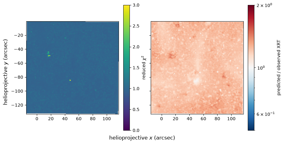
How well the DEM fits: the reduced \(\chi^2\) of each pixel, and the ratio of the XRT intensity the DEM predicts to the one observed. In every pixel the DEM predicts about 20% more than XRT observes. The inversion stops as soon as the reduced \(\chi^2\) reaches one, and with seven channels that can leave one of them, here XRT, further from its observation than its uncertainty; a smaller chi2_target fits it a little more closely. The DEM also predicts about 20% less 94 Å than observed, even with the correction of Boerner et al. [2014]. The two dark spots, where the ratio is largest, look like spots of contamination on the CCD which the Level 1 processing did not fill in. Only one pixel, two from the brightest one of the base, has a reduced \(\chi^2\) above 3. With the DEM starting at \(\log_{10} T = 5.5\), 119 do, 26 of them around the base of the jet, where 335 Å sees the most plasma of the transition region.

with astropy.visualization.quantity_support():
    fig, axs = plt.subplots(
        ncols=2,
        figsize=(9, 4.5),
        sharex=True,
        sharey=True,
        constrained_layout=True,
    )
    mesh = na.plt.pcolormesh(
        position_xrt,
        C=chi2,
        ax=axs[0],
        cmap="viridis",
        vmin=0,
        vmax=3,
    )
    fig.colorbar(mesh.ndarray.item(), ax=axs[0], label=r"reduced $\chi^2$")
    mesh = na.plt.pcolormesh(
        position_xrt,
        C=ratio,
        ax=axs[1],
        cmap="RdBu_r",
        norm=matplotlib.colors.LogNorm(vmin=0.5, vmax=2),
    )
    fig.colorbar(mesh.ndarray.item(), ax=axs[1], label="predicted / observed XRT")
    for ax in axs:
        ax.set_aspect("equal")
        ax.set_xlabel("")
        ax.set_ylabel("")
    fig.supxlabel("helioprojective $x$ (arcsec)")
    fig.supylabel("helioprojective $y$ (arcsec)")

Cross-calibration

This tutorial uses the response of XRT as xrtpy computes it, with no cross-calibration factor. Athiray and Winebarger [2024] predicted the intensity of a bright point in three XRT filters, Al_poly among them, from a DEM constrained by an X-ray spectrometer and AIA, and found that XRT observed about twice as much as predicted with the response of SolarSoft, so that its response would need a factor of about two. Del Zanna et al. [2022] predicted the intensity of Al_poly in an active region to within 20% from a DEM of the EUV Imaging Spectrometer and AIA, with no factor. The factor depends on the atomic data and the abundances behind each response, so it does not carry over from one response to another. To try a factor, multiply outputs_xrt by it before the inversion.