Filtergram#

class hinode.xrt.Filtergram(inputs=0, outputs=0, timedelta=<factory>, saturated=None, vignetting=None, uncertainty_map=None, leak=None, filter=None, coalignment=None, axis_time='time', axis_detector_x='detector_x', axis_detector_y='detector_y')[source]#

Bases: FunctionArray[ExplicitTemporalWcsPositionalVectorArray, ScalarArray]

A sequence of Level 1 images captured by the X-Ray Telescope (XRT) through one filter.

The images have been prepared by xrt_prep in SolarSoft, which subtracts the dark current, removes the read-out noise, corrects for vignetting, and divides by the exposure time, so the outputs are in DN per second.

Each image is one frame along axis_time, and its coordinates come from its own header, since the pointing changes from one image to the next. By default the pointing is corrected with the co-alignment database of SolarSoft from the cross-correlation of XRT with AIA [Yoshimura and McKenzie, 2015], so that the images line up with those of AIA, as coalignment records.

The time of each image, inputs.time, is the start of its exposure, DATE_OBS, as in the other sun-data packages, so the middle of each exposure is inputs.time + timedelta / 2.

Since 2012, visible light has leaked into XRT, which xrt_prep does not subtract. Load it with leak=True and subtract it with remove_leak(). The uncertainty of each pixel is found with uncertainty().

Examples

Load the Al_poly images captured while the EUV Snapshot Imaging Spectrograph (ESIS) was observing the Sun on 2019 September 30, and display the one with the most saturated pixels, which the jet called event E saturates.

import numpy as np
import matplotlib.pyplot as plt
import astropy.units as u
import astropy.visualization
import named_arrays as na
import hinode

# Load the images captured during the ESIS flight
images = hinode.xrt.open(
    time_start="2019-09-30T18:06:11",
    time_stop="2019-09-30T18:11:01",
    filter="Al_poly",
)

# Select the image with the most saturated pixels
num_saturated = images.saturated.sum(
    axis=(images.axis_detector_x, images.axis_detector_y),
)
image = images[np.argmax(num_saturated, axis=images.axis_time)]

# Display the image
unit = image.inputs.position.x.unit
with astropy.visualization.quantity_support():
    fig, ax = plt.subplots(figsize=(6, 6), constrained_layout=True)
    na.plt.pcolormesh(
        image.inputs.position.x,
        image.inputs.position.y,
        C=image.outputs,
        ax=ax,
        cmap="gray",
        norm="asinh",
        vmin=0 * u.DN / u.s,
        vmax=100 * u.DN / u.s,
    )
    ax.set_aspect("equal")
    ax.set_title(image.inputs.time.ndarray)
    ax.set_xlabel(f"helioprojective $x$ ({unit:latex_inline})")
    ax.set_ylabel(f"helioprojective $y$ ({unit:latex_inline})")

image.saturated.sum()

ScalarArray(ndarray=np.int64(6), shape={})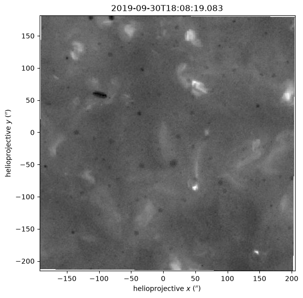

../_images/hinode.xrt.Filtergram_0_1.png

Attributes

`axes`	A `tuple` of `str` representing the names of each dimension of this array.
`axes_center`	Return keys corresponding to all input axes representing bin centers
`axes_flattened`	Combine `axes` into a single `str`.
`axes_vertex`	Return keys corresponding to all input axes representing bin vertices
`axis_detector_x`	The logical axis corresponding to changes in detector $x$-coordinate.
`axis_detector_y`	The logical axis corresponding to changes in detector $y$-coordinate.
`axis_time`	The logical axis corresponding to changes in time.
`broadcasted`	if this array has multiple components, broadcast them against each other.
`coalignment`	How the pointing of each image was found, numbered as `CALIBRATION_TYPE` of `xrt_read_coaldb.pro` in SolarSoft: 1 for the cross-correlation with AIA, 2 for a fit to the limb of the Sun in G-band, 3 for the Ultra Fine Sun Sensors (UFSS), 4 for a fit to the limb in X-rays, 6 for another method, and -1 for an image no database had an entry for, which keeps the center and the plate scale of its header but is still given the roll of `xrt_rollangle.pro`, or `None` if the pointing was not corrected.
`explicit`	Converts this array to an instance of `named_arrays.AbstractExplicitArray`.
`filter`	The filters the images were taken through, named as in `hinode.xrt.urls()`.
`indices`	Compute the index of each element of this array.
`inputs`	The inputs of the function.
`leak`	The visible light which leaks into each pixel and has not been subtracted, in DN per second, or `None` if the leak was not loaded.
`length`	L2-norm of this array.
`ndim`	Number of dimensions of the array.
`outputs`	The outputs of the function.
`saturated`	Whether each pixel is saturated, or charge has bled into it from a saturated pixel.
`shape`	The number of elements along each axis of the array.
`size`	Total number of elements in the array.
`type_abstract`	The `named_arrays.AbstractArray` type corresponding to this array.
`type_explicit`	The `named_arrays.AbstractExplicitArray` type corresponding to this array.
`uncertainty_map`	The uncertainty of each pixel due to the camera and to the processing of the image, in DN per second, as the uncertainty map of `xrt_prep`, `uncert_map`, gives it [Kobelski et al., 2014]: the error of the JPEG compression, of the dark subtraction, and of the vignetting correction, or `None` if the uncertainty was not loaded.
`value`	Returns a new array with its units removed, if they exist.
`vignetting`	The fraction of the light which reaches each pixel, which `xrt_prep` divided each image by, from the model of `nono_vignette.pro` in SolarSoft, or 1 for a dark frame, which `xrt_prep` does not correct for vignetting, or `None` if the uncertainty was not loaded.
`timedelta`	The exposure time of each image.

Methods

`__init__`([inputs, outputs, timedelta, ...])
`add_axes`(axes)	Add new singleton axes to this array.
`all`([axis, where])	Return `True` if all of the elements along the given axes are `True`.
`any`([axis, where])	Return `True` if any of the elements along the given axes are `True`.
`astype`(dtype[, order, casting, subok, copy])	Copy of the array cast to a specific data type.
`broadcast_to`(shape[, append])	A new view of this array with the specified shape.
`cell_centers`([axis, random, seed])	Convert an array from cell vertices to cell centers.
`combine_axes`([axes, axis_new])	Combine some of the axes of the array into a single new axis.
`copy`()	Create a deep copy of this array.
`copy_shallow`()	Create a shallow copy of this array.
`debroadcast`([axes])	Remove redundant axes introduced by broadcasting.
`from_fits`(path[, axis_time, ...])	Load one or more Level 1 XRT files taken through the same filter.
`from_scalar_array`(a[, like])	Constructs a new version of this array using `a` as the underlying data.
`from_time_range`(time_start, time_stop[, ...])	Download the Level 1 images which began during a given time range and were taken through a given filter, and construct an instance of `Filtergram`.
`gradient`(axis[, component, edge_order])	Differentiate the outputs with respect to the inputs along `axis`.
`index`(value[, axis])
`index_secant`(value[, axis])
`integrate`(axis[, component])	Integrate the outputs over the given input `axis` or axes.
`interp_linear`(item)	Linearly interpolate this array to find its value at the given fractional index.
`isel`(**item)	Index this array along named axes given as keyword arguments.
`max`([axis, initial, where])	The maximum value of this array along the given axes.
`mean`([axis, where])	The mean value of this array along the given axes.
`median`([axis])	The median value of this array along the given axes.
`min`([axis, initial, where])	The minimum value of this array along the given axes.
`ndindex`([axis_ignored])	An iterator that yields the index of each element of this array.
`pcolormesh`(axs, input_component_x, ...[, ...])	Plot a `FunctionArray` via `matplotlib.pyplot.pcolormesh()`.
`percentile`(q[, axis, out, overwrite_input, ...])	The requested percentile of this array along the given axes.
`ptp`([axis])	The peak-to-peak value of this array along the given axes.
`ratio_noise`(noise_photon[, where, ...])	The ratio of the variance of the noise measured in this sequence of images to the variance of `uncertainty()`.
`regrid`(inputs[, axis, method, weights])	Resample this function array onto a new set of input coordinates using `named_arrays.regridding.regrid()`.
`remove_leak`([scale])	Subtract the visible light leaking into each pixel, `leak`, from the images, as `xrt_synleaksub.pro` in SolarSoft does.
`replace`(**changes)	A method version of `dataclasses.replace()` for named arrays.
`reshape`(shape)	Reorganize this array into a new shape.
`rms`([axis, where])	The root-mean-square of this array along the given axes.
`std`([axis, where])	The standard deviation of this array along the given axes.
`sum`([axis, where])	The sum of each element of this array along the given axes.
`take_along_axis`(indices, axis)	Take values from this array by matching `indices` along `axis`.
`to`(unit[, equivalencies, copy])	Convert this array to a new unit.
`to_string`([prefix, multiline])	Convert this array instance to a string representation.
`to_string_array`([format_value, format_unit, ...])	Convert to an array of strings where each string has an appropriately-formatted unit attached to the value.
`to_value`(unit[, equivalencies])	The numerical value of this array, possibly in a different unit.
`transpose`([axes])	Reorder the axes of this array to the given sequence.
`uncertainty`(noise_photon)	The one-sigma uncertainty of each pixel, in DN per second.
`var`([axis, where])	The variance of this array along the given axes.
`vmr`([axis, where])	The variance-to-mean ratio of this array along the given axes.
`volume_cell`(axis)	Computes the n-dimensional volume of each cell formed by interpreting this array as a logically-rectangular grid of vertices.
`weights`(inputs[, axis, method])	Compute the resampling weights of this array using `named_arrays.regridding.weights()`.

Inheritance Diagram

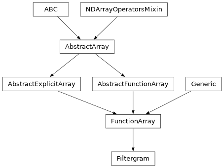
Parameters:

inputs (InputsT)
outputs (OutputsT)
timedelta (Quantity | AbstractScalar)
saturated (None | ScalarArray)
vignetting (None | ScalarArray)
uncertainty_map (None | ScalarArray)
leak (None | ScalarArray)
filter (None | str)
coalignment (None | ScalarArray)
axis_time (str)
axis_detector_x (str)
axis_detector_y (str)

classmethod from_fits(path, axis_time='time', axis_detector_x='detector_x', axis_detector_y='detector_y', leak=False, uncertainty=False, coalign='aia', directory=None, num_retry=5)[source]#

Load one or more Level 1 XRT files taken through the same filter.

The images are placed one after another along axis_time, in the order the files are given, and images smaller than the largest one are padded with NaN.

Parameters:

path (str | PathLike | Sequence[str | PathLike] | AbstractScalarArray) – A Level 1 XRT file, or a sequence of them, or an array of them such as the one hinode.xrt.download() returns, which is flattened.
axis_time (str) – The logical axis corresponding to changes in time.
axis_detector_x (str) – The logical axis corresponding to changes in detector $x$-coordinate.
axis_detector_y (str) – The logical axis corresponding to changes in detector $y$-coordinate.
leak (bool) – Whether to load the visible light leaking into each pixel, leak, from SolarSoft.
uncertainty (bool) – Whether to load vignetting and uncertainty_map, which uncertainty() needs. They are not loaded by default, since each takes as much memory as the images.
coalign (None | Literal['aia', 'ufss']) – Which co-alignment database of SolarSoft to correct the pointing of the images with, as xrt_read_coaldb.pro does, or None to keep the pointing of the headers. "aia" (the default) uses the cross-correlation of each image with AIA 335 Å [Yoshimura and McKenzie, 2015], and the Ultra Fine Sun Sensors (UFSS) of Hinode for an image it has no entry for, as xrt_read_coaldb.pro does with /aia_cc. "ufss" uses the UFSS alone, as it does by default. See coalignment.
directory (None | Path) – The directory to place the downloaded images of the leak and the co-alignment databases in. If None (the default), hinode.directory_default is used.
num_retry (int) – The number of times to try to connect to the server for the co-alignment databases.

Raises:

ValueError – If xrt_prep did not divide an image by its exposure time, which it does only if asked to with its /normalize keyword, if the history of a file does not record the value xrt_prep set the saturated pixels to, if leak is True and SolarSoft has no image of the leak for the filter and the time of an image, if uncertainty is True and the compression of an image is not known, or if coalign is not "aia", "ufss", or None.
ConnectionError – If a file of the co-alignment databases an image needs has not been downloaded before and cannot be downloaded, in which case coalign=None keeps the pointing of the headers.

Return type:

Filtergram

Notes

The pixels with no data, which xrt_prep sets to -999, are set to NaN.

The headers give the roll of each image as CROTA2 rather than as a PC matrix, and it is converted to one the way Calabretta and Greisen [2002] describe for that older keyword.

xrt_prep has already corrected the pointing of the Level 1 files with the UFSS, so the center of an image moves only with "aia", the default. Either database also gives each image the roll xrt_rollangle.pro gives it now. Since the attitude anomaly of 2021 December 27, the roll is interpolated in a database which grows as the roll is measured, and some of the files xrt_prep made before it existed have a roll in their header which is more than a degree from it, and up to 23 degrees during the anomaly. Like xrt_read_coaldb.pro, the correction places the center the database gives at pixel NAXIS // 2 + 0.5, counted from one, with the plate scale of the X-ray or the G-band images.

The files of the databases are downloaded to directory the first time an image needs them. They are downloaded again when the listing of the server shows they have changed, and the listings and the database of the roll are checked again after a day for an image later than they reach, and after a month for any image. If the server cannot be reached, the copies downloaded before are used, with a warning. A warning is also given for an image the database of the roll does not reach yet, since it is extrapolated, as xrt_rollangle.pro extrapolates it, and the measurements reach the server days after the images.

classmethod from_scalar_array(a, like=None)#

Constructs a new version of this array using a as the underlying data.

Parameters:

a (float | Quantity | AbstractScalarArray) – Anything that can be coerced into an instance of named_arrays.AbstractScalarArray.
like (None | Self) – Optional reference object. If provided, the result will be defined by this object.

Return type:

Self

classmethod from_time_range(time_start, time_stop, filter='Al_poly', axis_time='time', axis_detector_x='detector_x', axis_detector_y='detector_y', directory=None, overwrite=False, num_retry=5, leak=False, uncertainty=False, coalign='aia')[source]#

Download the Level 1 images which began during a given time range and were taken through a given filter, and construct an instance of Filtergram.

Parameters:

time_start (str | Time) – The earliest start time of the images.
time_stop (str | Time) – The time before which an image must begin.
filter (str) – The filters the images were taken through, named as in hinode.xrt.urls().
axis_time (str) – The logical axis corresponding to changes in time.
axis_detector_x (str) – The logical axis corresponding to changes in detector $x$-coordinate.
axis_detector_y (str) – The logical axis corresponding to changes in detector $y$-coordinate.
directory (None | Path) – The directory to place the downloaded files in. If None (the default), hinode.directory_default is used.
overwrite (bool) – Boolean flag controlling whether to download files which are already in directory.
num_retry (int) – The number of times to try to connect to the server.
leak (bool) – Whether to load the visible light leaking into each pixel, leak.
uncertainty (bool) – Whether to load vignetting and uncertainty_map, which uncertainty() needs.
coalign (None | Literal['aia', 'ufss']) – Which co-alignment database of SolarSoft to correct the pointing of the images with, as xrt_read_coaldb.pro does, or None to keep the pointing of the headers. "aia" (the default) uses the cross-correlation of each image with AIA 335 Å [Yoshimura and McKenzie, 2015], and the Ultra Fine Sun Sensors (UFSS) of Hinode for an image it has no entry for, as xrt_read_coaldb.pro does with /aia_cc. "ufss" uses the UFSS alone, as it does by default. See coalignment.

Raises:

ValueError – If coalign is not "aia", "ufss", or None, which is checked before any image is downloaded, or for the reasons from_fits() gives.
ConnectionError – For the reasons from_fits() gives.

Return type:

Filtergram

add_axes(axes)#

Add new singleton axes to this array.

Parameters:: axes (str | Sequence[str]) – Either a single axis name or a sequence of axis names add to this array.
Return type:: FunctionArray

See also

named_arrays.add_axes(): A functional version of this method.

all(axis=None, where=<no value>)#

Return True if all of the elements along the given axes are True.

Parameters:

axis (None | str | Sequence[str]) – The logical axis or axes along which the operation is computed.
where (Self) – An optional mask which selects which elements to be considered.
self (Self)

Return type:

Self

See also

numpy.all(): A functional version of this method.

any(axis=None, where=<no value>)#

Return True if any of the elements along the given axes are True.

Parameters:

axis (None | str | Sequence[str]) – The logical axis or axes along which the operation is computed.
where (Self) – An optional mask which selects which elements to be considered.
self (Self)

Return type:

Self

See also

numpy.any(): A functional version of this method.

astype(dtype, order='K', casting='unsafe', subok=True, copy=True)#

Copy of the array cast to a specific data type.

Equivalent to numpy.ndarray.astype().

Parameters:

dtype (str | dtype | type)
order (str)
subok (bool)
copy (bool)

Return type:

FunctionArray

broadcast_to(shape, append=False)#

A new view of this array with the specified shape.

Parameters:

shape (dict[str, int]) – The shape of the new array.
append (bool) – If True, shape will be appended to the current shape of this array before broadcasting.
self (Self)

Return type:

Self

See also

named_arrays.broadcast_to(): A functional version of this method.

cell_centers(axis=None, random=False, seed=None)#

Convert an array from cell vertices to cell centers.

Parameters:

axis (None | str | Sequence[str]) – The axes of the array to average over.
random (bool) – If true, select a random point within each cell instead of the geometric center.
seed (None | int) – The seed of the random sampling, which has an effect only where random is true. If None (the default), the sampling differs from one call to the next, and anything computed from it cannot be reproduced.

Return type:

AbstractExplicitArray

combine_axes(axes=None, axis_new=None)#

Combine some of the axes of the array into a single new axis.

Parameters:

axes (None | Sequence[str]) – The axes to combine into a new axis
axis_new (None | str) – The name of the new axis

Return type:

Array with the specified axes combined

copy()#

Create a deep copy of this array.

Parameters:: self (Self)
Return type:: Self

copy_shallow()#

Create a shallow copy of this array.

Parameters:: self (Self)
Return type:: Self

debroadcast(axes=None)#

Remove redundant axes introduced by broadcasting.

Parameters:

axes (None | str | Sequence[str]) – The axes to consider removing. If None (the default), every axis of this array is considered. Axes not present in this array are ignored.
self (Self)

Return type:

Self

See also

named_arrays.debroadcast(): A functional version of this method.

gradient(axis, component=None, edge_order=1)#

Differentiate the outputs with respect to the inputs along axis.

This is the counterpart to integrate(): where that one sums the outputs against a measure computed from the inputs, this one divides the difference of the outputs by the difference of the inputs.

The result has the same inputs as this array, and its outputs are the derivative, so the units of the result are those of the outputs divided by those of the differentiation variable.

If component is None, the inputs themselves are the differentiation variable, and they must be a scalar.
If component is a str, that named sub-element of the inputs is the variable, and it must be a scalar.

A center axis, where the inputs are samples, differentiates the outputs against those samples directly. A vertex axis, where the inputs are bin edges and so has one more input than output, differentiates against the cell centers, which is where the outputs live.

Parameters:

axis (str) – The logical axis to differentiate along.
component (None | str) – The named input sub-element which is the differentiation variable. If None, the inputs themselves are the variable.
edge_order (int) – The order of the one-sided differences used at the two ends of axis, either 1 or 2. The interior always uses second-order central differences.

Raises:

ValueError – If axis is not an axis of this array, if the differentiation variable is not a scalar or does not vary along axis, or if there are too few points along axis for the given edge_order.

Return type:

FunctionArray

See also

integrate(): The counterpart of this method, which sums the outputs against the inputs rather than dividing by them.
numpy.gradient(): The numpy function this method backs.

Notes

Unlike numpy.gradient(), the differentiation variable may vary along axes other than axis, which is what a distorted grid gives, since the differences are taken elementwise.

Examples

Differentiate a parabola, whose derivative is a straight line.

Second-order edges are asked for, since the first-order ones of the default are inexact wherever the function curves.

import numpy as np
import astropy.units as u
import named_arrays as na

x = na.linspace(0, 2, axis="x", num=5) * u.mm

f = na.FunctionArray(
    inputs=x,
    outputs=np.square(x / u.mm) * u.ph,
)

f.gradient("x", edge_order=2)

FunctionArray(
    inputs=ScalarArray(
        ndarray=[0. , 0.5, 1. , 1.5, 2. ] mm,
        shape={'x': 5},
    ),
    outputs=ScalarArray(
        ndarray=[0., 1., 2., 3., 4.] ph / mm,
        shape={'x': 5},
    ),
)

index(value, axis=None)#

Parameters:

self (Self)
value (Self)
axis (None | str | Sequence[str])

Return type:

dict[str, Self]

index_secant(value, axis=None)#

Parameters:

self (Self)
value (Self)
axis (None | str | Sequence[str])

Return type:

dict[str, Self]

integrate(axis, component=None)#

Integrate the outputs over the given input axis or axes.

The differential measure is computed from the inputs via AbstractArray.volume_cell():

If component is None, the whole input is used as the integration variable and len(axis) must match the dimensionality of the inputs (one for a scalar, two for a Cartesian2dVectorArray, etc.).
If component is a str, that named sub-element of the inputs (a scalar or a sub-vector) supplies the measure, and len(axis) must match its dimensionality.

A vertex axis (where the inputs represent bin edges) is integrated with a Riemann sum, while a center axis (where the inputs represent samples) is integrated with the trapezoidal rule; mixing the two in a single call is supported. The integrated axes are removed from the outputs and collapsed in the inputs by averaging.

Parameters:

axis (str | Sequence[str]) – The logical axis or axes to integrate over.
component (None | str) – The named input sub-element supplying the integration variable. If None, the whole input is used.

Return type:

FunctionArray

Examples

Integrate a constant function over a 1D domain.

import numpy as np
import astropy.units as u
import named_arrays as na

f = na.FunctionArray(
    inputs=na.ScalarLinearSpace(0, 2, axis="x", num=101) * u.nm,
    outputs=na.ScalarArray(np.full(101, 3.0), axes=("x",)) * u.ph,
)

f.integrate("x")

FunctionArray(
    inputs=ScalarArray(
        ndarray=1. nm,
        shape={},
    ),
    outputs=ScalarArray(
        ndarray=6. nm ph,
        shape={},
    ),
)

interp_linear(item)#

Linearly interpolate this array to find its value at the given fractional index.

Parameters:: item (dict[str, AbstractArray]) – A fractional index at which to evaluate the array.
Return type:: FunctionArray

isel(**item)#

Index this array along named axes given as keyword arguments.

This is a convenience wrapper around __getitem__(): a.isel(x=0) is equivalent to a[dict(x=0)].

Since keyword-argument names must be valid Python identifiers, axes whose names are not valid identifiers can only be indexed using the dict form, a[{...}].

Parameters:

item (int | slice | AbstractArray) – The index to apply along each named axis.
self (Self)

Return type:

AbstractExplicitArray

max(axis=None, initial=<no value>, where=<no value>)#

The maximum value of this array along the given axes.

Parameters:

axis (None | str | Sequence[str]) – The logical axis or axes along which the operation is computed.
initial (ArrayLike) – The initial value of the minimum, required if where provided.
where (Self) – An optional mask which selects which elements to be considered.
self (Self)

Return type:

Self

See also

numpy.max(): A functional version of this method.

mean(axis=None, where=<no value>)#

The mean value of this array along the given axes.

Parameters:

axis (None | str | Sequence[str]) – The logical axis or axes along which the operation is computed.
where (Self) – An optional mask which selects which elements to be considered.
self (Self)

Return type:

Self

See also

numpy.mean(): A functional version of this method.

median(axis=None)#

The median value of this array along the given axes.

Parameters:: axis (None | str | Sequence[str]) – The logical axis or axes along which the operation is computed.

See also

numpy.median(): A functional version of this method.

min(axis=None, initial=<no value>, where=<no value>)#

The minimum value of this array along the given axes.

Parameters:

axis (None | str | Sequence[str]) – The logical axis or axes along which the operation is computed.
initial (ArrayLike) – The initial value of the minimum, required if where provided.
where (Self) – An optional mask which selects which elements to be considered.
self (Self)

Return type:

Self

See also

numpy.min(): A functional version of this method.

ndindex(axis_ignored=None)#

An iterator that yields the index of each element of this array.

Parameters:

axis_ignored (None | str | Sequence[str]) – The of the array to ignore when generating the iterator.
self (Self)

Return type:

Iterator[dict[str, int]]

See also

named_arrays.ndindex(): A functional version of this method.

pcolormesh(axs, input_component_x, input_component_y, input_component_row=None, input_component_column=None, index=None, output_component_color=None, **kwargs)#

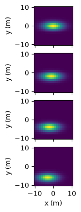
Plot a FunctionArray via matplotlib.pyplot.pcolormesh().

FunctionArray.pcolormesh() takes in an axes object, or array of axes objects, along with components to be plotted along the x and y plot axes (input_component_x and input_component_y). Additional components can be tiled along subplot row/column and are specified in input_component_row and input_component_column.

import named_arrays as na
import numpy as np
import astropy.units as u
import matplotlib.pyplot as plt

position = na.Cartesian2dVectorLinearSpace(
    start=-10,
    stop=10,
    axis=na.Cartesian2dVectorArray(
        x='position_x',
        y='position_y',
    ),
    num=21,
) * u.m

x_width = 5 * u.m
y_width = 2 * u.m
velocity = 1 * u.m/u.s
time = na.ScalarLinearSpace(
    start=0 * u.s,
    stop=3 * u.s,
    num=4,
    axis='time'
)

intensity = np.exp(-(((position.x + velocity*time)/x_width) ** 2 + ((position.y + 2*velocity*time)/y_width)** 2))
scene = na.FunctionArray(
    inputs=position,
    outputs=intensity,
)

fig, axs = plt.subplots(
    nrows=scene.outputs.shape['time'],
    squeeze=False,
    sharex=True,
    subplot_kw=dict(aspect='equal'),
)
scene.pcolormesh(
    axs=axs,
    input_component_x='x',
    input_component_y='y',
    input_component_row='time',
)

../_images/hinode.xrt.Filtergram_3_0.png

Parameters:

axs (ndarray)
input_component_x (str)
input_component_y (str)
input_component_row (None | str)
input_component_column (None | str)
index (None | dict[str, int])
output_component_color (None | str)
kwargs (Any)

percentile(q, axis=None, out=None, overwrite_input=False, method='linear', keepdims=False)#

The requested percentile of this array along the given axes.

Parameters:

q (int | float | Quantity | Self) – The percentile to compute.
axis (None | str | Sequence[str]) – The logical axis or axes along which the operation is computed.
out (None | Self) – An optional output array in which to place the result.
overwrite_input (bool) – Whether to overwrite the input array.
method (str) – How to interpolate the result.
keepdims (bool) – A boolean flag indicating whether to keep the reduced dimensions.
self (Self)

See also

numpy.percentile(): A functional version of this method.

ptp(axis=None)#

The peak-to-peak value of this array along the given axes.

Parameters:

axis (None | str | Sequence[str]) – The logical axis or axes along which the operation is computed.
self (Self)

Return type:

Self

See also

numpy.ptp(): A functional version of this method.

ratio_noise(noise_photon, where=True, threshold=<Quantity 10. DN / s>, gap=<Quantity 25. s>, clip=5, num_iteration=3)[source]#

The ratio of the variance of the noise measured in this sequence of images to the variance of uncertainty().

The noise is measured from the difference between each image and the next. Where the Sun barely changes between the two, the difference is the noise of both images, and dividing it by their uncertainties,

\[z = \frac{I_2 - I_1}{\sqrt{\sigma_1^2 + \sigma_2^2}},\]

gives a quantity whose variance is the ratio.

An image is compared with the next only if the next begins after it and within gap of it, with the same exposure time, and with the same plate scale and pointing, so that the first pixel of each lands within a pixel of the same place on the Sun, since otherwise the same pixel of the two images sees different parts of the Sun. Of those pixels, only the ones selected by where in both images are used, which are not saturated in either, and whose mean signal over the two images is fainter than threshold, since brighter ones are more likely to change. The mean is independent of the difference for noise of the same variance in both images, so selecting on it barely biases the ratio, while selecting on the signal of each image would leave out the largest differences near threshold. What bias is left comes from uncertainty() following the noise of the signal it is found from, and is a few percent for pixels at threshold.

The ratio is first estimated from the median of $z^2$, which the outliers barely move, as that median over the median of the square of Gaussian noise. Cosmic rays and changes of the Sun are then left out by clipping $z$ at clip times the square root of the ratio, and the ratio is found again as the mean of $z^2$ left, which is repeated num_iteration times.

The noise of the images of XRT is less than uncertainty() predicts, since the charge of each photon diffuses into the neighboring pixels and the compression of the images removes some of the noise, so this ratio can scale uncertainty() to the noise measured. It is measured in faint pixels, and compression removes less of the noise of brighter ones. The errors of the dark subtraction and of the vignetting correction in uncertainty_map are the same in both images and cancel in their difference, so the ratio is of the noise which changes from one image to the next, and scaling all of uncertainty() by it scales those errors too, which in faint pixels are a small part of it.

Parameters:

noise_photon (Quantity | AbstractScalar) – The factor which sets the photon noise, as in uncertainty().
where (bool | AbstractScalar) – The pixels to measure the noise in, which should leave out any which change between images, such as those of a jet. It may differ from one image to the next.
threshold (Quantity) – The mean signal of two images above which their pixels are left out.
gap (Quantity) – The longest time between the starts of two images compared.
clip (float) – How many times the measured noise a difference may be before it is left out.
num_iteration (int) – How many times to clip the differences.

Returns:

The ratio, one for each entry of any axes other than axis_time, axis_detector_x, and axis_detector_y, such as those of noise_photon.

Return type:

ratio

Raises:

ValueError – If there are fewer than two images along axis_time, or if no pair of images compared has a pixel to measure the noise in, for some entry of the other axes.

Examples

The ratio for the Al_poly images captured while ESIS was observing the Sun, with the photon noise of plasma at 2 MK, away from the jet called event E.

import numpy as np
import astropy.units as u
import named_arrays as na
import hinode

images = hinode.xrt.open(
    time_start="2019-09-30T18:06:11",
    time_stop="2019-09-30T18:11:01",
    leak=True,
    uncertainty=True,
).remove_leak()

time = images.inputs.time.ndarray[0]
response = hinode.xrt.temperature_response("Al_poly", time)
variance = hinode.xrt.temperature_response("Al_poly", time, variance=True)

# The temperature closest to 2 MK
index = dict(
    filter=0,
    temperature=int(np.argmin(np.abs(response.inputs.ndarray - 2 * u.MK))),
)
noise_photon = (variance.outputs / response.outputs)[index]

# Every pixel except those of the jet
where = na.ScalarArray.ones(images.outputs[dict(time=0)].shape) > 0
where[dict(detector_x=slice(172, 300), detector_y=slice(80, 208))] = False

images.ratio_noise(noise_photon, where=where)

ScalarArray(ndarray=np.float64(0.15269618329306375), shape={})

regrid(inputs, axis=None, method='multilinear', weights=None)#

Resample this function array onto a new set of input coordinates using named_arrays.regridding.regrid().

Parameters:

inputs (AbstractArray) – The new input coordinates on which to resample the outputs.
axis (None | str | tuple[str]) – The logical axes of the input over which to resample.
method (Literal['multilinear', 'conservative']) – The resampling method to use.
weights (None | tuple[AbstractScalar, dict[str, int], dict[str, int]]) – Optional weights which can be computed in advance using weights() to greatly speed repeated resampling of the same inputs.

Return type:

Self

See also

weights(): If you need to resample the same coordinates more than once.

remove_leak(scale=1)[source]#

Subtract the visible light leaking into each pixel, leak, from the images, as xrt_synleaksub.pro in SolarSoft does.

The result has no leak left to subtract, so its leak is zero, and subtracting it again changes nothing.

Parameters:: scale (float) – The factor to multiply the leak by before subtracting it, kfact in xrt_synleaksub.pro.
Return type:: Filtergram

Examples

The median signal of the Al_poly images captured while ESIS was observing the Sun, before and after the leak is subtracted.

import hinode

images = hinode.xrt.open(
    time_start="2019-09-30T18:06:11",
    time_stop="2019-09-30T18:11:01",
    leak=True,
)

axes = (images.axis_detector_x, images.axis_detector_y)

print(images.outputs.median(axes))
print(images.remove_leak().outputs.median(axes))

ScalarArray(
    ndarray=[3.2920074, 3.2923155, 3.2906594, 3.2862515, 3.2961397, 3.2970128, 3.2968717, 3.297009 , 3.3026195,
             3.316657 , 3.3035352, 3.2999496, 3.3096128] DN / s,
    shape={'time': 13},
)
ScalarArray(
    ndarray=[2.3720171, 2.3704367, 2.3692963, 2.3650246, 2.3737645, 2.3745394, 2.3756442, 2.3775065, 2.3808184,
             2.3961992, 2.381784 , 2.3793426, 2.3882186] DN / s,
    shape={'time': 13},
)

replace(**changes)#

A method version of dataclasses.replace() for named arrays.

Parameters:: changes – The fields of the dataclass to be overwritten
Return type:: Self

reshape(shape)#

Reorganize this array into a new shape.

Parameters:

shape (dict[str, int]) – The new shape of the array, must be compatible with this array.
self (Self)

Return type:

Self

rms(axis=None, where=<no value>)#

The root-mean-square of this array along the given axes.

Parameters:

axis (None | str | Sequence[str]) – The logical axis or axes along which the operation is computed.
where (Self) – An optional mask which selects which elements to be considered.
self (Self)

Return type:

Self

std(axis=None, where=<no value>)#

The standard deviation of this array along the given axes.

Parameters:

axis (None | str | Sequence[str]) – The logical axis or axes along which the operation is computed.
where (Self) – An optional mask which selects which elements to be considered.
self (Self)

Return type:

Self

See also

numpy.std(): A functional version of this method.

sum(axis=None, where=<no value>)#

The sum of each element of this array along the given axes.

Parameters:

axis (None | str | Sequence[str]) – The logical axis or axes along which the operation is computed.
where (Self) – An optional mask which selects which elements to be considered.
self (Self)

Return type:

Self

See also

numpy.sum(): A functional version of this method.

take_along_axis(indices, axis)#

Take values from this array by matching indices along axis.

Parameters:

indices (AbstractArray) – The integer indices to take along axis.
axis (str) – The axis of this array along which the values are taken.
self (Self)

Return type:

Self

See also

named_arrays.take_along_axis(): A functional version of this method.

to(unit, equivalencies=[], copy=True)#

Convert this array to a new unit.

Equivalent to astropy.units.Quantity.to().

Parameters:

unit (UnitBase) – New unit of the returned array
equivalencies (None | list[tuple[Unit, Unit]]) – A list of equivalence pairs to try if the units are not directly convertible.
copy (bool) – Boolean flag controlling whether to copy the array.

Return type:

FunctionArray

to_string(prefix=None, multiline=None)#

Convert this array instance to a string representation.

Parameters:

prefix (None | str) – the length of this string is used to align the output
multiline (None | bool) – flag which controls if the output should be spread over multiple lines.

Return type:

array represented as a str

to_string_array(format_value='%.2f', format_unit='latex_inline', pad_unit='$\\,$')#

Convert to an array of strings where each string has an appropriately-formatted unit attached to the value.

Parameters:

format_value (str) – The string used to format the numeric value of each element.
format_unit (str) – The string used to format the units of each element.
pad_unit (str) – The string used to add horizontal space between the value and unit.

to_value(unit, equivalencies=[])#

The numerical value of this array, possibly in a different unit.

Equivalent to astropy.units.Quantity.to_value().

Parameters:

unit (UnitBase) – New unit of the returned array
equivalencies (None | list[tuple[Unit, Unit]]) – A list of equivalence pairs to try if the units are not directly convertible.

Return type:

FunctionArray

transpose(axes=None)#

Reorder the axes of this array to the given sequence.

Parameters:

axes (None | Sequence[str]) – The new axis ordering of this array.
self (Self)

Return type:

Self

See also

numpy.transpose(): The numpy version of this method.

uncertainty(noise_photon)[source]#

The one-sigma uncertainty of each pixel, in DN per second.

This is the photon noise of the signal combined with the uncertainty due to the camera and the processing of the image, uncertainty_map,

\[\sigma^2 = \frac{F \max(I, 0)}{V t} + \sigma_\text{map}^2,\]

where $I$ is the signal of the pixel, outputs, $V$ is the vignetting, vignetting, $t$ is the exposure time, timedelta, and $F$ is the factor which sets the photon noise [Kobelski et al., 2014].

The photons of each wavelength give a different signal $s$, so the variance of the signal due to the counting of the photons is $F = \langle s^2 \rangle / \langle s \rangle$ times the signal before the vignetting correction and the normalization. $F$ depends on the spectrum, so it is given. For plasma at one temperature it is the ratio of the response of hinode.xrt.temperature_response() with variance=True to the response without it, and for a differential emission measure (DEM) it is the ratio of the two responses each weighted by the DEM. Subtract the leak first, with remove_leak(), since visible photons give much less signal each than X-rays.

Parameters:: noise_photon (Quantity | AbstractScalar) – The factor which sets the photon noise, $\langle s^2 \rangle / \langle s \rangle$, in DN per photon, which may vary from pixel to pixel.
Return type:: ScalarArray

Examples

The median relative uncertainty of the Al_poly images captured while ESIS was observing the Sun, with the photon noise of plasma at 2 MK.

import numpy as np
import astropy.units as u
import hinode

images = hinode.xrt.open(
    time_start="2019-09-30T18:06:11",
    time_stop="2019-09-30T18:11:01",
    leak=True,
    uncertainty=True,
).remove_leak()

time = images.inputs.time.ndarray[0]
response = hinode.xrt.temperature_response("Al_poly", time)
variance = hinode.xrt.temperature_response("Al_poly", time, variance=True)

# The temperature closest to 2 MK
index = dict(
    filter=0,
    temperature=int(np.argmin(np.abs(response.inputs.ndarray - 2 * u.MK))),
)
noise_photon = (variance.outputs / response.outputs)[index]

uncertainty = images.uncertainty(noise_photon)

axes = (images.axis_detector_x, images.axis_detector_y)
(uncertainty / images.outputs).median(axes)

ScalarArray(
    ndarray=[0.28826082, 0.28828306, 0.2883124 , 0.28866826, 0.28804463, 0.28804776, 0.28788095, 0.2879158 , 0.28758778,
             0.34223147, 0.28762664, 0.28773509, 0.28719184] ,
    shape={'time': 13},
)

var(axis=None, where=<no value>)#

The variance of this array along the given axes.

Parameters:

axis (None | str | Sequence[str]) – The logical axis or axes along which the operation is computed.
where (Self) – An optional mask which selects which elements to be considered.
self (Self)

Return type:

Self

See also

numpy.var(): A functional version of this method.

vmr(axis=None, where=<no value>)#

The variance-to-mean ratio of this array along the given axes.

Parameters:

axis (None | str | Sequence[str]) – The logical axis or axes along which the operation is computed.
where (Self) – An optional mask which selects which elements to be considered.

volume_cell(axis)#

Computes the n-dimensional volume of each cell formed by interpreting this array as a logically-rectangular grid of vertices.

Note that this method is usually only used for sorted arrays.

If self is a scalar, this method computes the length of each edge, and is equivalent to numpy.diff(). If self is a 2d vector, this method computes the area of each quadrilateral, and if self is a 3d vector, this method computes the volume of each cuboid.

Parameters:: axis (None | str | Sequence[str]) – The axis or axes defining the logically-rectangular grid. If self is a physical scalar, there should only be one axis. If self is a physical vector, there should be one axis for each component of the vector.
Return type:: AbstractScalar

weights(inputs, axis=None, method='multilinear')#

Compute the resampling weights of this array using named_arrays.regridding.weights(). The output of this method is designed to be used by regrid().

Parameters:

inputs (AbstractArray) – The new input coordinates on which to resample the outputs.
axis (None | str | tuple[str]) – The logical axes of the input over which to resample.
method (Literal['multilinear', 'conservative']) – The resampling method to use.

Return type:

tuple[AbstractScalar, dict[str, int], dict[str, int]]

See also

regrid(): A method designed to use these weights.

property axes: tuple[str, ...]#

A tuple of str representing the names of each dimension of this array.

Must have the same length as the number of dimensions of this array.

property axes_center: tuple(str)#: Return keys corresponding to all input axes representing bin centers

property axes_flattened: str#

Combine axes into a single str.

This is useful for functions like numpy.flatten() which returns an array with only one dimension.

property axes_vertex: tuple(str)#: Return keys corresponding to all input axes representing bin vertices

axis_detector_x: str = 'detector_x'#: The logical axis corresponding to changes in detector $x$-coordinate.

axis_detector_y: str = 'detector_y'#: The logical axis corresponding to changes in detector $y$-coordinate.

axis_time: str = 'time'#: The logical axis corresponding to changes in time.

property broadcasted: FunctionArray#

if this array has multiple components, broadcast them against each other.

Equivalent to a.broadcast_to(a.shape).

coalignment: None | ScalarArray = None#: How the pointing of each image was found, numbered as CALIBRATION_TYPE of xrt_read_coaldb.pro in SolarSoft: 1 for the cross-correlation with AIA, 2 for a fit to the limb of the Sun in G-band, 3 for the Ultra Fine Sun Sensors (UFSS), 4 for a fit to the limb in X-rays, 6 for another method, and -1 for an image no database had an entry for, which keeps the center and the plate scale of its header but is still given the roll of xrt_rollangle.pro, or None if the pointing was not corrected.

property explicit: FunctionArray#: Converts this array to an instance of named_arrays.AbstractExplicitArray.

filter: None | str = None#: The filters the images were taken through, named as in hinode.xrt.urls().

property indices: dict[str, ScalarArrayRange]#

Compute the index of each element of this array.

See also

named_arrays.indices(): A functional version of this method.

inputs: InputsT = 0#: The inputs of the function.

leak: None | ScalarArray = None#

The visible light which leaks into each pixel and has not been subtracted, in DN per second, or None if the leak was not loaded.

Since the entrance filters of XRT began to tear in 2012, visible light has leaked into the X-ray filters [Takeda et al., 2016]. The leak is found from the image of the leak SolarSoft has for the filter and the stray-light phase of each image, which xrt_synleaksub.pro selects, cut out and resampled to the part of the CCD each image covers. It is zero before the first tear, on 2012 May 9, for dark frames, which no light reaches, for files whose history says that SolarSoft has already subtracted it, and once remove_leak() has subtracted it.

The images of the leak were taken with Hinode pointed near the center of the Sun, and the pattern of the leak changes with the pointing, so it is most reliable for images near the center of the Sun. It also varies by about 10% with the contamination of the CCD.

property length: FunctionArray#: L2-norm of this array.

property ndim: int#: Number of dimensions of the array. Equivalent to numpy.ndarray.ndim.

outputs: OutputsT = 0#: The outputs of the function.

saturated: None | ScalarArray = None#

Whether each pixel is saturated, or charge has bled into it from a saturated pixel.

xrt_prep sets every pixel above the saturation level, 2500 DN, to exactly that level before correcting for vignetting and dividing by the exposure time, and records the level in the history of the file, so a pixel is saturated if the product of its value, the exposure time, and the vignetting function of xrt_prep is at least the recorded level. The level is lowered by 0.01% to allow for the rounding of the exposure time in the header and of the values stored in the file.

The CCD bleeds the charge of a saturated pixel along its columns, so the pixels just above and just below each saturated pixel, which xrt_prep grades as possibly affected by “bloom/bleed”, are marked as well.

property shape: dict[str, int]#: The number of elements along each axis of the array. Analogous to numpy.ndarray.shape but represented as a dict where the keys are the axis names and the values are the axis sizes.

property size: int#: Total number of elements in the array. Equivalent to numpy.ndarray.size

timedelta: Quantity | AbstractScalar#: The exposure time of each image.

property type_abstract: Type[AbstractFunctionArray]#: The named_arrays.AbstractArray type corresponding to this array.

property type_explicit: Type[FunctionArray]#: The named_arrays.AbstractExplicitArray type corresponding to this array.

uncertainty_map: None | ScalarArray = None#

The uncertainty of each pixel due to the camera and to the processing of the image, in DN per second, as the uncertainty map of xrt_prep, uncert_map, gives it [Kobelski et al., 2014]: the error of the JPEG compression, of the dark subtraction, and of the vignetting correction, or None if the uncertainty was not loaded.

It does not include the photon noise, which depends on the spectrum of the plasma, so the whole uncertainty is found with uncertainty().

It differs from the map of xrt_prep in three ways. xrt_prep finds the error of the JPEG compression from the range of the signal of the Level 0 image in each block of 8 by 8 pixels, and here the signal is found from the Level 1 image instead, by undoing the vignetting correction and the division by the exposure time. xrt_prep gives an image which was not compressed with a loss an error of 1 DN for its compression, from the value of -1 by which get_jpeg_unc.pro signals that it has no model for it, and here such an image has no error for its compression. xrt_prep also includes an empirical model of the error of its Fourier filtering of the read-out noise, which is left out here.

property value: FunctionArray#

Returns a new array with its units removed, if they exist.

The family is preserved, so a vector returns a vector and a function array returns a function array, but the result is always explicit: an implicit array materializes into its family’s explicit type.

vignetting: None | ScalarArray = None#: The fraction of the light which reaches each pixel, which xrt_prep divided each image by, from the model of nono_vignette.pro in SolarSoft, or 1 for a dark frame, which xrt_prep does not correct for vignetting, or None if the uncertainty was not loaded.